Old Models, New Frameworks: Reviving GANs with Flax

08 Dec, 2023

The purpose of this blog post is to guide you through the implementation of a Generative Adversarial Network (GAN) with Flax.

My journey into this topic began with JAX, a new framework by Google that combines a Numpy-like interface with advanced features like Autograd and XLA compilation. Moreover, it is built on the principles of functional programming, meaning functions are purely dependent on input parameters, free from external state influences. For those intrigued by the inner workings of JAX, I highly recommend exploring its documentation, which offers insights on pure functions and random number generation.

While you can build neural networks directly with JAX, the ecosystem around it, particularly Flax for architecture construction and Optax for optimization and loss functions, makes the development process more enjoyable.

Our focus here will be on implementing a simple GAN. Don’t worry if you’re new to GANs: we will go through the theory and the practical aspects, drawing insights from Chapter 26 of the great Probabilistic Machine Learning: Advanced Topics.

A Bit of Theory on GANs

Generative Adversarial Networks (GANs), introduced in the seminal paper by Ian Goodfellow et al. in 2017, have revolutionized the field of machine learning and laid the foundations for the modern generative models.

The Need for Two Networks

Imagine you want to generate new data from an unknown distribution $p^*$, from which we only have some examples.

In traditional machine learning tasks, we commonly employ static loss functions to evaluate the performance of neural networks. These loss functions compare the network’s prediction with the ground truth and provide a metric for assessing the ‘goodness’ of the network’s outputs. These metrics play a crucial role in the backpropagation process, guiding the network in adjusting its parameters for improved performance.

In the context of generative models, evaluating the quality of generated samples presents a unique challenge. Ideally, to determine if a sample is of high quality, one would require access to the true distribution $p^*$ and compute some distance measure $\mathcal D(p^*,q)$ from the true distribution to our generated data, denoted as $q$. However, in practice, having access to $p^*$ is often impractical or impossible.

Rather than relying on a static, predefined loss functios, GANs consists in two networks: the generator that produces the samples, and a discriminator, which serves as a dynamic loss function. The generator’s goal is to produce data so convincing that the discriminator, trained to distinguish real data from fake, gets fooled. As the generator evolves and improves its output, the discriminator adapts and refines its ability to detect fakes. In particular:

The Generator $G_\theta$ model takes as input random noise $q(\mathbf z)$, such as a gaussian $q(\mathbf z)\sim\mathcal N (0,1)$, passes the noise trough some layers and produces a density $q_\theta(\mathbf x)$ on the output space.
The Discriminator $D_\phi$ is a classifier. Its role is to discern whether a sample is from $p^*$ or a generator product.

Training the Networks

The training process consists of two phases:

First Phase: The discriminator $D_\phi$ is trained for $K$ steps in which we sample noise from $q(\mathbf z)$ and true examples from the dataset. The discriminator is optimized to distinguish real data apart from fake data, therefore we optimize the usual cross-entropy loss:

$$ \min_\phi -\overbrace{y\log [D_\phi(\mathbf x)]}^{\textrm{real data}} -\overbrace{(1-y)\log[1-D_\phi(G_\theta(\mathbf z))]}^{\textrm{fake data}} $$

Second Phase: After the first phase we should have a good discriminator that we can use as a loss to improve the generator. Therefore we sample noise from $q(\mathbf z)$ and we maximize the chance to fool the discriminator: $$\max_\theta-\log[1-D_\phi(G_\theta(\mathbf z))]$$ However, when the generator performs poorly, hence $D_\phi(G_\theta(\mathbf z))\approx 0$, the loss nears zero, leading to vanishingly small gradients. This problem can be solved by using an alternative formulation with better gradients, called “non-saturating loss”: $$\min_\theta -\log[D_\phi(G_\theta(\mathbf z))]$$

Implementation

Data Generation

In our example, we will consider a simple distribution as our dataset, where using GANs might seem like overkill but serves as a good example.

dataset

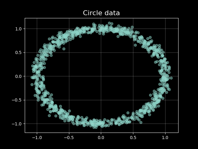
In the following code, we can see data generation and dataloader. Notice that we need to handle the random number generation ourselves, as we did for the generator. More on this in the documentation here.

from typing import Tuple
import numpy as np
import jax
import jax.numpy as jnp
from jax import random
import tensorflow as tf


def generate_circle_data(
    key: random.PRNGKey, n_samples: int, r: int = 1, noise: float = 0.05
):
    subkey1, subkey2, subkey3 = random.split(key, 3)
    theta = jax.random.uniform(
        key=subkey1, shape=(n_samples,), minval=0, maxval=2 * jnp.pi
    )
    x_noise = jax.random.normal(key=subkey2, shape=(n_samples,)) * noise
    x = r * jnp.cos(theta) + x_noise
    y_noise = jax.random.normal(key=subkey3, shape=(n_samples,)) * noise
    y = r * jnp.sin(theta) + y_noise
    return jnp.stack([x, y], axis=1)


def get_dataloader(dataset: Tuple[np.ndarray, ...], batch_size: int):
    return (
        tf.data.Dataset.from_tensor_slices(dataset)
        .shuffle(2000)
        .batch(batch_size, drop_remainder=True)
        .as_numpy_iterator()
    )

Generator and Discriminator

We’ll use Flax’s linen module for defining our models. It offers a PyTorch-like class instantiation but the key difference is that we’re defining a dataclass, which doesn’t hold the network’s parameters itself, but only serves as a “storage” of functions to apply.

import jax
import flax.linen as nn

class Generator(nn.Module):
    hidden_channels: int
    batch_size: int

    @nn.compact
    def __call__(self, z_rng):
	    # Latent (for which we need a random number generator)
        z = jax.random.normal(z_rng, (self.batch_size, 2))
        z = nn.Dense(self.hidden_channels)(z)
        z = nn.leaky_relu(z)
        z = nn.Dense(self.hidden_channels)(z)
        z = nn.leaky_relu(z)
        # Data in the sample space
        x = nn.Dense(2)(z)
        return x

class Discriminator(nn.Module):
    hidden_channels: int

    @nn.compact
    def __call__(self, x):
        x = nn.Dense(self.hidden_channels)(x)
        x = nn.leaky_relu(x)
        x = nn.Dense(self.hidden_channels)(x)
        x = nn.leaky_relu(x)
        x = nn.Dense(2)(x)
        return x

The nn.compact decorator allows to definition of the network directly in the __call__method. This approach simplifies the model creation process, though we could define layers separately as well (check out setup vs compact for more info on that). You might have noticed that the generator __call__method requires a random number generator as input. This is because random number generation in JAX is handled directly by the user. This may sound like a lot of effort, but it allows you to take control over the randomness generation by forcing you to think carefully about what is going on.

I also defined two functions that will come in handy to use functools.partial later in the code:

def generator_model(hidden_channels, batch_size):
    return Generator(hidden_channels=hidden_channels, batch_size=batch_size)


def discriminator_model(hidden_channels):
    return Discriminator(hidden_channels=hidden_channels)

Training Loop

The training loop consists of initializing the models and defining the training steps for both the generator and discriminator. First, we use functools.partial to derive functions with certain arguments pre-filled, then we need to initialize the parameters of the networks by using the init method of the linen module.

# We use partial to pass the hidden_channels and batch_size to the model
generator = partial(
	generator_model,
	hidden_channels=cfg.hidden_dims,
	batch_size=cfg.batch_size
)

discriminator = partial(
	discriminator_model,
	hidden_channels=cfg.hidden_dims
)

# Init parameters by passing a dummy input
generator_params = generator().init(rngs=gen_key, z_rng=gen_key)
discriminator_params = discriminator().init(
	disc_key, jnp.ones((cfg.batch_size, 2), dtype=jnp.float32)
)

Then, we instantiate two TrainState dataclasses, which are useful for having model functions, parameters and optimizers in one place without having to pass all of them as arguments to the training functions:

# Instantiate training states
gen_state = train_state.TrainState.create(
	apply_fn=generator().apply,
	params=generator_params,
	tx=optax.adam(learning_rate=cfg.gen_lr),
)

disc_state = train_state.TrainState.create(
	apply_fn=discriminator().apply,
	params=discriminator_params,
	tx=optax.adam(learning_rate=cfg.disc_lr),
)

The training process follows the phases discussed earlier:


def train_step(gen_state, disc_state, batch, rng, cfg):
	# Generate random numbers
    rng, gen_key, disc_key = random.split(rng, 3)

	# First phase: Discriminator steps
    for _ in range(cfg.disc_steps):
        # We need to re-initialize the key for the latent space,
        # otherwise the generator will always generate the same data
        rng, gen_key = random.split(rng)
        disc_state, disc_loss = discriminator_step(
            gen_state, disc_state, batch, disc_key
        )

	# Second phase: Generator step
	gen_state, gen_loss = generator_step(gen_state, disc_state, gen_key)
    return gen_state, disc_state, gen_loss, disc_loss, rng

Let us take a closer look at the discriminator step:

@jit
def discriminator_step(gen_state, disc_state, batch, latent_key):
    fake_data = gen_state.apply_fn(gen_state.params, latent_key)

    def loss_fn(params):
        fake_logits = disc_state.apply_fn(params, fake_data)
        real_logits = disc_state.apply_fn(params, batch)

        fake_loss = optax.sigmoid_binary_cross_entropy(
            fake_logits, jnp.zeros_like(fake_logits)
        )
        real_loss = optax.sigmoid_binary_cross_entropy(
            real_logits, jnp.ones_like(real_logits)
        )
        loss = jnp.mean(fake_loss + real_loss)
        return loss

    loss, grads = value_and_grad(loss_fn)(disc_state.params)
    disc_state = disc_state.apply_gradients(grads=grads)
    return disc_state, loss

The @jit decorator here compiles the function for faster execution. The loss function is defined inside the step and takes as input only the parameters of the discriminator. This is useful to apply value_and_grad, which computes the gradient of the loss with respect to its parameters and returns its value. Finally, we update the parameters in the state by using apply_gradients.

The generator step is similar, with a different loss function:

@jit
def generator_step(gen_state, disc_state, latent_key):
    def loss_fn(params):
        fake_data = gen_state.apply_fn(params, latent_key)
        fake_logits = disc_state.apply_fn(disc_state.params, fake_data)

        # In the non-saturating loss, we want to maximize the probability that
        # the discriminator classifies the fake data as real
        loss = -jnp.mean(jnp.log(nn.sigmoid(fake_logits)))
        return loss

    loss, grads = value_and_grad(loss_fn)(gen_state.params)
    gen_state = gen_state.apply_gradients(grads=grads)
    return gen_state, loss

These ingredients are enough to train our GAN. Below the final result at the end of the training process:

training

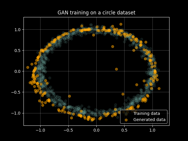
The full code is available on GitHub. At the end of the training process you should see a nice GIF that shows the evolution of the generator’s output.

Conclusion

We saw how to implement a GAN in Flax, by first going into some theoretical review and then diving into some of the peculiarities of this framework. I hope you found this exploration as useful and interesting as it was for me to write it. Your feedback, comments, and critiques are welcome.

References

Kevin P. Murphy (2023). Probabilistic Machine Learning: Advanced Topics. MIT Press.